Dealing with heavy-tailed noise: the Japanese bracket cost function

Update (April 18, 2016): For a more detailed mathematical analysis, see this post.

Update (April 17, 2016): What I call the Japanese bracket cost function below seems to already be known as the Pseudo-Huber loss function. See this Wikipedia page for references.

Background and motivation

Many machine-learning problems can be formulated as minimizing a training cost plus a regularization cost. The simplest example is linear regression, in which for training data $X$ and labels $y$, one seeks to solve the problem:

$\min_{W, b} \textrm{cost}(X \cdot W + b - y) + C \cdot\textrm{reg_cost}(W) \,.$

Here $W$ and $b$ are the coefficients to be fitted and $C$ is a hyperparameter that controls the strength of the regularization.

Two widely-used cost functions are the squared $\ell^2$ norm and the $\ell^1$ norm. If $z$ is an $n$-dimensional vector, these are given by:

$\begin{align} \frac{1}{n} ||z||_{\ell^2}^2 &= \frac{1}{n} \sum_{i=1}^n |z_i|^2 \,, \label{l2} \\ \frac{1}{n} ||z||_{\ell^1} &= \frac{1}{n} \sum_{i=1}^n |z_i| \,. \label{l1} \end{align}$

For example, the squared-$\ell^2$ norm is used as both the cost and regularization cost in Ridge regression, and in Lasso regression, the squared-$\ell^2$ norm is still used for the training cost, but the $\ell^1$ norm is used for regularization. (The motivation for using $\ell^1$ in this context is to make $W$ sparse.)

The purpose of this article is:

To raise awareness that for heavy-tailed noise the squared $\ell^2$ norm is not a suitable cost function: least squares regression will likely fail.
To introduce the Japanese bracket cost function that does work well for heavy-tailed noise. It is a smooth interpolation between the $\ell^1$ and squared $\ell^2$ costs.

Heavy-tailed noise and least-squares regression

Let’s distort samples from the line $y = 3 + 50x$ by some Cauchy heavy-tailed noise.

import numpy as np
x = np.linspace(0, 100, 500)
y_noisy = 3 + 50 * x + 20 * np.random.standard_cauchy(500)

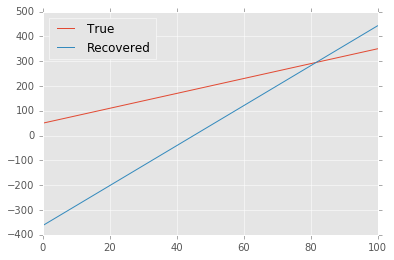
Here is an example of what we get if we try to recover $y$ from the noisy data using least-squares regression (i.e. squared $\ell^2$ training cost):

         True: 50.000 + 3.000 * x
    Recovered: -362.910 + 8.056 * x

Disastrous fit using least-squares regression

That doesn’t look so good. The problem is that the quadratic growth of the cost function makes it too sensitive to the outliers.

Upshot: Least-squares regression is a disaster for Cauchy noise.

Heavy-tailed noise and the $\ell^1$ norm

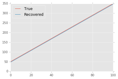
So what if we use the $\ell^1$ norm instead? It only grows linearly, so it should be much less sensitive to the outliers. Indeed, the results look much better:

         True: 50.000 + 3.000 * x
    Recovered: 47.083 + 3.007 * x

$Much better fit using $\ell^1$ norm$

The Japanese bracket cost

The solution is to use the Japanese bracket

$\langle z \rangle := \sqrt{1 + |z|^2}$

instead of the absolute value function. (This name and notation are widespread in the partial differential equations literature, but I have been unable to trace their origin.) The point is that

$\langle z \rangle \approx \begin{cases} 1 + \frac12 |z|^2 \,, & \text{for $z \ll 1$}\,, \\ |z| \,, & \text{for $z \gg 1$}\,. \end{cases}$

Thus, $\langle z \rangle - 1$ is a smooth function that interpolates between quadratic behavior for small $z$ and linear growth for large $z$.

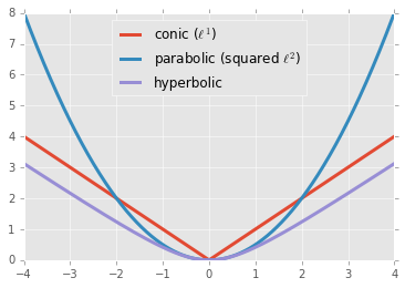
Geometrically, it is nice to think about these cost functions in terms of quadric (hyper)surfaces: $y = \frac12 |z|^2$ defines a paraboloid, whereas $y = |z|$ defines a cone, which is a degenerate hyperboloid. The Japanese bracket comes from solving $y^2 = 1 + |z|^2$, which is a nondegenerate hyperboloid.

Cone, parabola, and hyperbola

With this in mind and in analogy with $\eqref{l2}$ and $\eqref{l1}$, we define the Japanese bracket cost to be

$\textrm{japanese}(z) = \frac{\eta^2}{n} \sum_i \left( \sqrt{ 1 + \left( \frac{|z_i|}{\eta} \right)^2 } - 1 \right) \,,$

where $\eta$ is a positive scale parameter. In principle, $\eta$ can be optimized just like any other hyperparameter: Just make sure to use a metric like $\ell^1$ for the cross-validation that is independent of $\eta$. In practice, if the training data is pre-scaled, $\eta$ can simply be taken as, say, $0.1$.)

Choosing somewhat arbitrarily $\eta = 10$ for the non-scaled data in this post, here finally are the results of the fit using the Japanese bracket cost. They are comparable with the $\ell^1$ results.

         True: 50.000 + 3.000 * x
    Recovered: 47.135 + 2.998 * x

Equally good fit using Japanese bracket cost

Code

The regressions in this post were computed using a custom scikit-learn estimator. Please see flexible_linear.py and heavytail.ipynb in this repository.

Credit

For more on the observation that least-squares regression is not suitable for heavy-tailed noise, see, e.g., Schick and Mitter (PDF).

I learned about this issue from my mentor George Bordakov when I was an intern at Schlumberger. We introduced the Japanese bracket cost here (paywall) to deal with heavy-tailed noise in well-log sharpening (a geophysical inverse problem).